How To Switch X and Y Axis In Excel
Learning how to switch the x-axis and y-axis in Excel will save you a lot of trouble and stress!
Most graphs and charts in Excel, except for pie charts, have an x and y axes where data in a column or row are plotted. So if it does not display the worksheet data on the axis that you prefer, you can quickly change the way that data is plotted.
For example, if rows of data are displayed on the vertical (category) axis, but you want them to be displayed on the horizontal (value) axis instead, you can switch rows to columns so that the data is displayed in the chart the way that you prefer.
Microsoft Excel’s chart and graph features are so advanced that you can literally swap the series value on the axes without touching the original data on the spreadsheet. In this article, we’ll show you how to switch x and y axes in Excel.
Table of Contents
Learn to Switch X and Y Axis in Excel
Microsoft Excel is a powerful spreadsheet software that will let you store data and make calculations on it. You can then visualize the data using built-in charts and graphs.
However, there are times when switching the value series of the chart’s axes can get confusing. And if you don’t know how to do it, your only choice is to exchange the columns or values manually.
The X-Axis and Y-Axis
By definition, the x and y axes are the two perpendicular lines on a graph where the labels are put.
Below is an example of an Excel line chart that shows the X and Y axes taken from SpreadSheeto.com
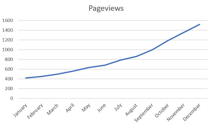
In the example above, the x-axis is the horizontal line where the months are named. In the example above, the y-axis is the vertical line with the numbers.
How to switch the axes
If you don’t know how to switch the axes, you would’ve deleted the chart and copy-pasted your contents within columns B and C to exchange the values manually.
There’s a better way than that where you don’t need to change any values.
First, right-click on either of the axes in the chart and click ‘Select Data’ from the options.
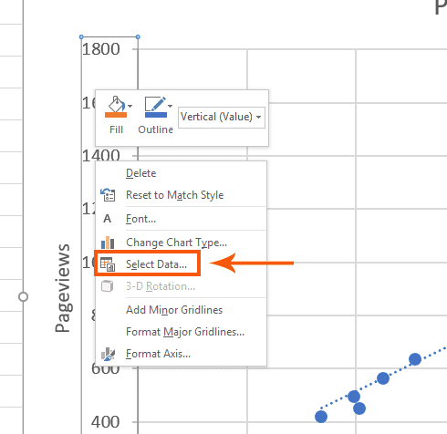
A new window will open.
Click ‘Edit’.
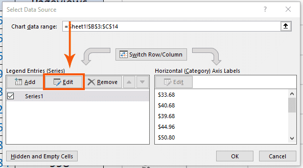
Another window will open where you can exchange the values on both axes.
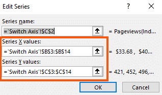
Now all you need to do is exchange the content of the ‘Series X values’ and ‘Series Y values’. You can use notepad and copy the values. Then, simply paste them on each form.
Your goal is to change the values from this:
To this:
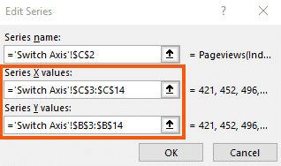
Once you do that, the value series on the axes would be swapped.
You’ll notice that we didn’t change any values on the spreadsheet data at all. All we did was customized the chart.
How do you swap x and y axis in Excel?
In this tutorial, you will see how to switch the X and Y axis in an excel graph. Watch the step by step all of the things you need to do to swap these around on the graph. The method described in the video works for a scatter plot, bar graph, or line graph in exactly the same way. The key is to use the edit data option.
How do you flip the Axis in Excel?
Rotating the Excel chart has these basic 5 steps:
- Select or click on the chart to see Chart Tools on the Ribbon.
- Select the Format tab.
- Head to the Chart Elements drop down list and pick Vertical (Value) Axis.
- Click the Format Selection button to see the Format Axis window.
- On the Format Axis window tick the Values in reverse order checkbox.