How to Edit Legend in Excel
Legends are crucial for understanding any chart in Excel. Every time you create a graph or plot data, it creates a legend. Before we talk about editing the legend in Excel, let’s talk about adding legend to an Excel graph in case you encounter one without it.:
Table of Contents
How to Add a Legend to an Excel chart
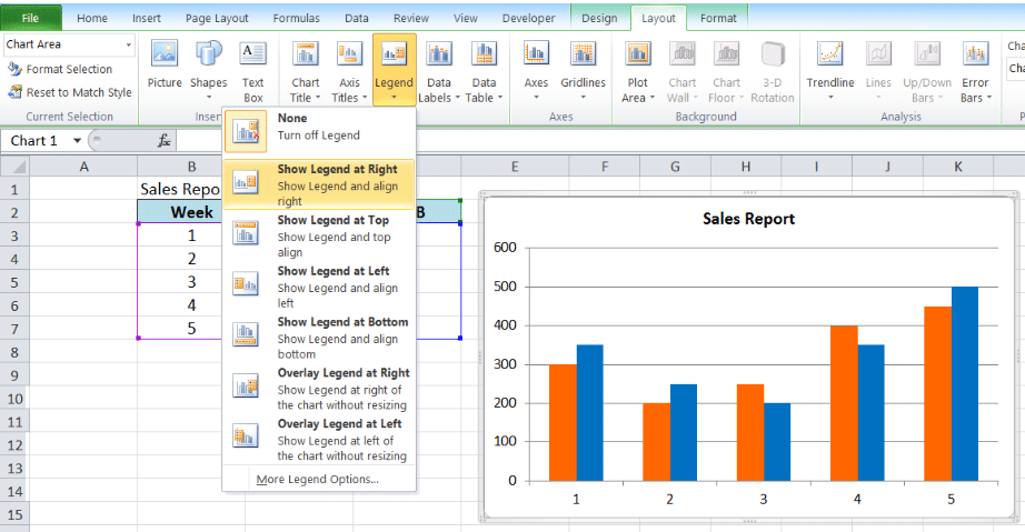
Step 1. Click on the chart
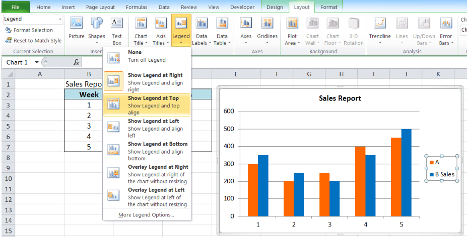
Step 2. Select the Layout tab, and then click on Legend
Step 3. From the Legend drop-down menu, choose the position to display the legend.
Case in point: Select Show Legend at Right
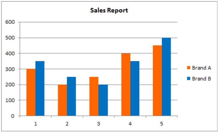
The legend appears on the right side of the graph.
An Excel chart’s legend can be edited by changing its name/position or format.
How to change legend name?
Here’s how you can change legend name:
- Change series name in Select Data
- Change legend name
Change Series Name in Select Data
1. Right-click anywhere on the chart and click Select Data
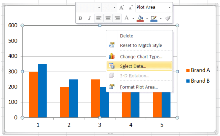
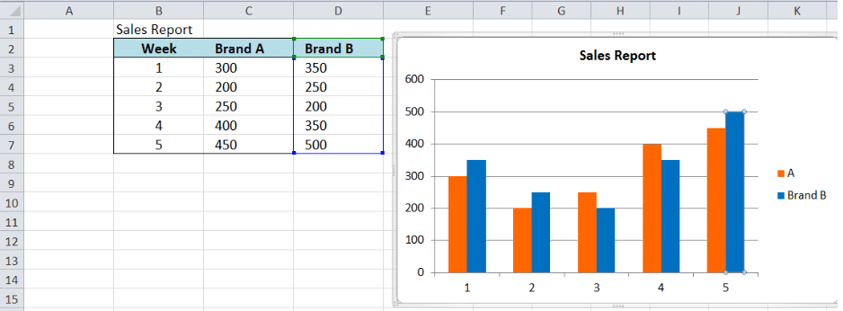
2. Select the series Brand A and click Edit
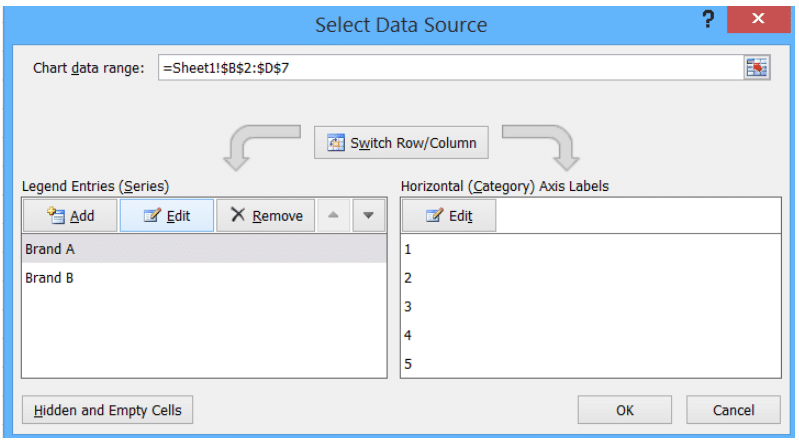
This leads to the Edit Series dialog box to pop-up.
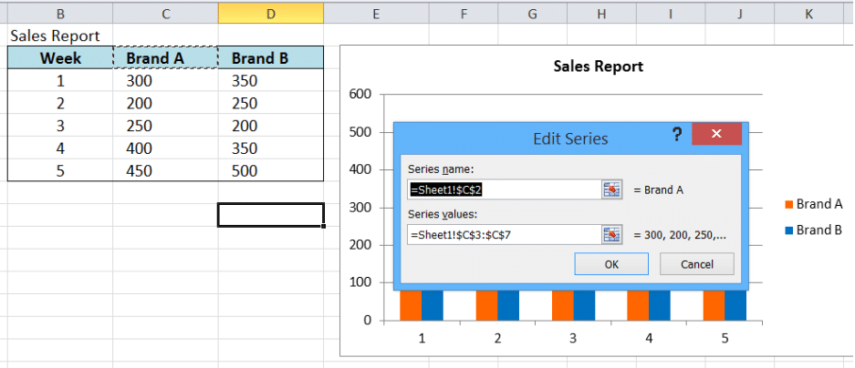
3. Delete the current entry “=Sheet1!$C$2” in series name and enter “A” into the text box.
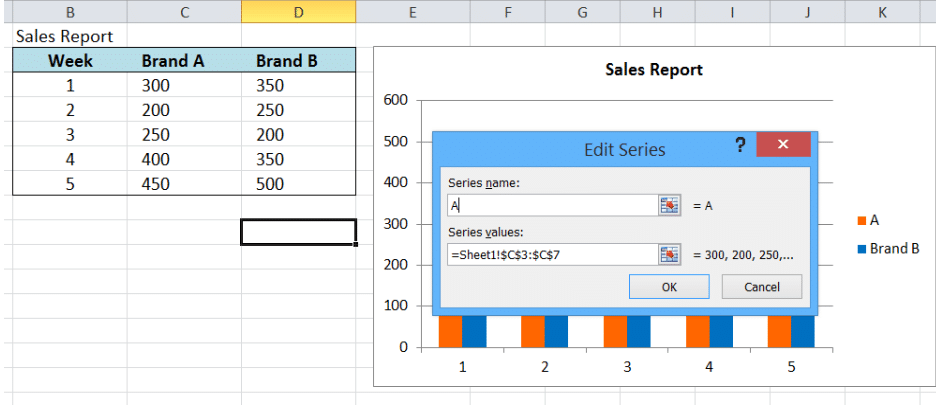
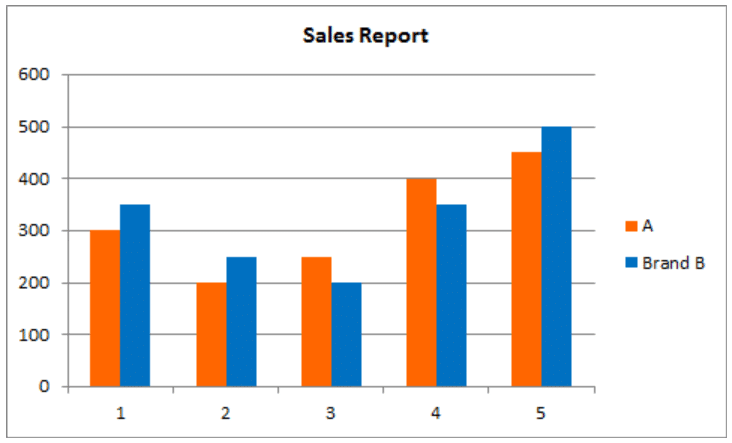
The legend name has now been changed to “A”.
Change legend name
1. First, we must determine the cell that contains the legend name for our chart by clicking the chart. As shown below, the column chart for Brand B is linked to cells D2:D7.
2. Since D2 contains the legend name, select D2 and type the new legend name “B Sales”.
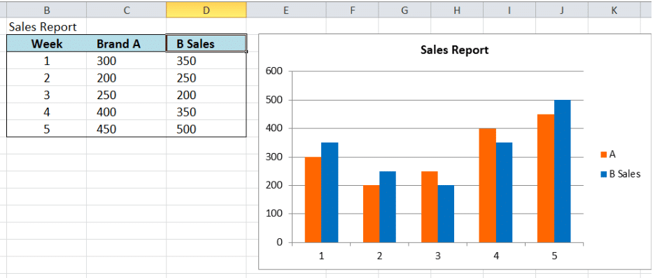
As shown above, the legend name on the chart is instantly updated from “Brand B” to “B Sales”.
How to edit legend name?
Legends can be customized by changing the layout, position or format.
How to change legend position?
Changing legend position on Excel is quite easy. Just click the chart, then click the Layout tab. Under Legend, choose the preferred position from the drop-down menu.
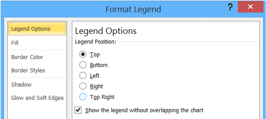
How to edit legend format?
Legend format can be changed by right clicking the legend and selecting Format Legend.
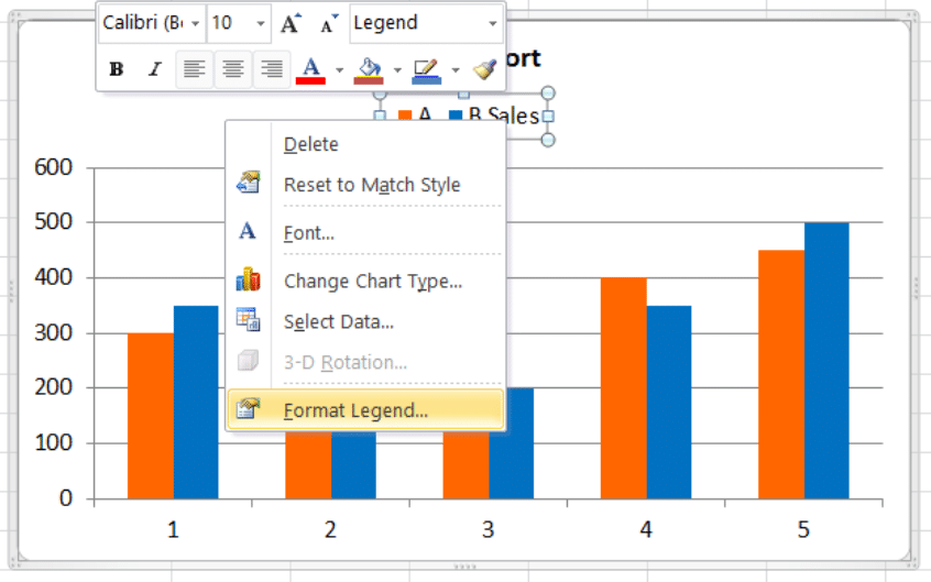
In the ensuing Format Legend dialog box, you can make a lot of changes to the legend as shown in the picture below.